Interpretation of Subsurface Hydrocarbon Shows
Tim T. Schowalter, Paul D. Hess
Search and Discovery Article #40001 (1999)
|
Hydrocarbons occur in the subsurface in four modes: (1) continuous phase oil or gas, (2) isolated droplets of oil or gas, (3) dissolved hydrocarbons, and (4) associated with kerogenous rocks. All of these modes of occurrence can result in what is described as a subsurface hydrocarbon "show." Each show type has markedly different implications to exploration and must be differentiated as the first step in show interpretation. Only continuous phase occurrences of oil and gas indicate that a trapped and potentially producible accumulation of hydrocarbons has been discovered. Free oil or gas recovery from the formation or subsurface hydrocarbon saturations of greater than 55% indicates a continuous phase occurrence. Continuous phase shows can be interpreted quantitatively. The static hydrocarbon column downdip from a continuous phase occurrence can be calculated from one well bore if the subsurface oil or gas saturation, capillary properties, hydrocarbon-water interfacial tension, oil density, and water density of the reservoir are known. Producing wells are by definition continuous phase oil or gas, and estimates of oil-water or gas-water contacts from normally available exploration data are practical and reasonably accurate based on a documented field study. Continuous phase oil or gas can extend either updip or downdip from a commercial reservoir. These continuous phase shows can also be interpreted quantitatively to determine how large an oil or gas column is required downdip to explain the show. By this method it can be determined whether an exploratory well penetrated the updip waste zone or downdip transition zone of an oil or gas field. Field studies illustrate that quantitative show interpretation of noncommercial shows can provide reliable estimates of the downdip hydrocarbon column. This type of data can be used in a systematic manner to explore for subtle stratigraphic and combination traps. |
Interpretation of subsurface hydrocarbon shows can be approached in three logical steps. The first step is to determine the physical mode of occurrence of the hydrocarbons encountered when drilling an exploratory well. Hydrocarbons in the subsurface can occur in four distinct physical modes: (1) continuous phase oil or gas, (2) isolated droplets of oil or gas, (3) molecular-scale dissolved hydrocarbons, or (4) associated with oil or gas source rocks. The significance of these modes of occurrence is that only continuous phase oil or gas is potentially producible by conventional petroleum production techniques. The three other modes of occurrence cannot produce oil or gas economically, but are often identified as "shows." The critical first step in interpreting shows in petroleum exploration is to determine if the hydrocarbons are potentially producible continuous phase oil or gas.
If a hydrocarbon show can be identified as continuous phase oil or gas, the second step (Figure 1) is to assess whether the observed hydrocarbons can be produced to the borehole at economic rates and quantities. Well bores are evaluated as to economic producibility by logs, formation tests, cores, and sample examination. If a show is interpreted to be economically productive, casing is run and a completion is attempted. Historical drilling data suggest that the identification of commercial productivity is difficult, as many dry holes with shows are later recompleted as commercial wells. This problem of evaluation of producibility is further complicated by continually changing petroleum economics. Many shows that could be commercial under current economic conditions may have been evaluated as noncommercial when they were drilled and consequently were plugged and abandoned. This paper does not address the problem of economic evaluation of well bores.
Step three in the interpretation procedure for subsurface shows is extrapolation of the significance of the show beyond the well bore. If a wildcat show is completed as a commercial producer, the obvious question is: what is the maximum extent of this newly discovered field? For structural traps, the limits of the newly discovered field are usually inferred from subsurface or seismic mapping of simple or fault closures. Limits of stratigraphic traps are estimated from mapping of stratigraphic closure or by prediction of reservoir distribution.
A more direct method of estimating the limits of a field is available when "show" data from a producing well bore are interpreted quantitatively. Schowalter (1979) and others have suggested that the downdip limits of an oil or gas accumulation can be estimated from hydrocarbon show data in a single well bore by using the principles of secondary hydrocarbon migration and entrapment. An analogous method to calculate lateral seal or fault seal capacity from core data has been suggested by Smith (1966) and Berg (1975).
In the following discussion, the terms "oil" and "gas" can be used interchangeably. A quantitative estimate of the downdip oil-water contact in an oil field can be made if the capillary properties, oil saturation, oil-water interfacial tension, oil-water densities, and hydrodynamic conditions are known. If subsurface saturations cannot be calculated, estimates of the maximum and minimum oil column that must be present downdip from the well can be made by comparing the minimum oil column required to explain a 10% saturation in oil or gas-saturated rocks and water-saturated rocks in the reservoir zone. This extrapolation of hydrocarbon show data beyond the well bore is useful in field development and exploration.
Shows in noncommercial wells can also be interpreted quantitatively. The minimum oil column necessary to migrate hydrocarbons through the water-saturated pore space of any oil-saturated rock or to explain a given oil saturation can be calculated based on the same principles (Smith, 1966; Berg, 1975; Schowalter, 1979). If the oil show can be identified as a continuous phase oil occurrence, the show is directly associated with a trapped oil column whose downdip limits can be estimated by this method.
This paper is composed of two main parts. Part one includes the development of a show classification and the recognition of show types. Part two reports case history attempts to quantify the oil or gas column downdip from oil and gas shows.
CLASSIFICATION OF HYDROCARBON PHYSICAL MODES OF OCCURRENCE
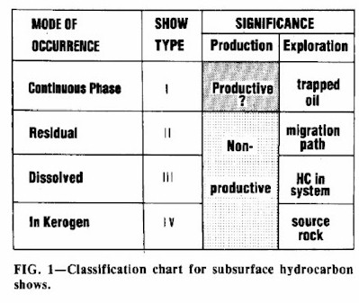
As stated in the introduction, oil or gas can occur in the subsurface as: (1) continuous phase oil or gas in water-saturated porous rocks; (2) isolated droplets of oil or gas in water-saturated porous rocks similar to waterflood residual oil or gas occurrence (hydrocarbon residues are also included in this group, which will be called residual oil shows for convenience); (3) molecular-scale dissolved hydrocarbons; and (4) hydrocarbons incorporated in kerogen or directly associated with oil or gas source rocks. The physical modes for the convenience of classification are referred to as type I, type II, type III, and type IV, respectively, in Figure 1. Any of these physical modes can be described during the drilling operation as subsurface hydrocarbon "show."
A subsurface hydrocarbon show is defined as any indication of oil or gas observed while drilling or completing a well. The hydrocarbons can be directly seen in drilling fluids, in core or cutting samples, and in formation or production tests, or may be seen indirectly as "anomalies" on wireline logs. Each show type will be discussed as to the physical distribution of the hydrocarbons, how this physical mode of occurrence can be manifested as a hydrocarbon show, and the production and exploration significance of each show type.
Continuous Phase Shows (Type I)
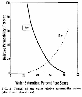
A continuous phase hydrocarbon occurrence is a filament of oil or gas with a continuous connection through the pore network of a water-saturated porous rock. The minimum pore volume saturation of oil or gas needed to establish a continuous hydrocarbon phase through the pore network of a water-saturated rock is approximately 10% (Schowalter, 1979). Thus, the percent of pore volume saturated by hydrocarbons in a continuous phase occurrence can be as low as 10%; maximum saturations can be as high as 90%. The ability of oil or gas to flow in a continuous phase mode of occurrence will depend on the percentage of the pore space saturated by oil versus water (Arps, 1964). This relationship is referred to as relative permeability and a typical oil-water relative permeability curve is illustrated in Figure 2. In reservoir-quality rocks, continuous phase shows are thought to represent trapped accumulations of hydrocarbons. Continuous phase occurrence may or may not be commercially productive. Economic producibility will depend on the reservoir qualities of the rock, the depth, the oil saturation, and corresponding relative permeability.
Figure 1. Classification chart for subsurface hydrocarbon shows.
Figure 2. Typical oil and water relative permeability curves (after Core Laboratories).
Isolated droplets of oil or gas are referred to as type II, or residual shows, in the classification. Water displacement residual hydrocarbons are isolated droplets of oil or gas in the pores of a rock like those left in a depleted reservoir. Another type of residual show is a hydrocarbon residue. Hydrocarbon residues include viscous films of oil or oil-degradation products coating the grains of rock, or solid to semisolid bitumen or oil (devolatilized, pyrolyzed, or otherwise degraded) in the pores. Hydrocarbon residues are immobile films or particles, whereas water-displacement residuals are liquid or gaseous hydrocarbons.
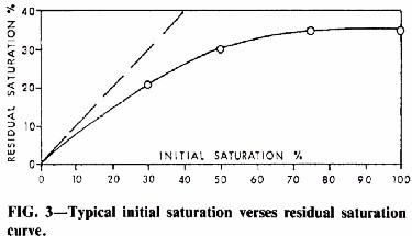
Water-displacement residual hydrocarbons can be created by: (1) oil or gas migration through a reservoir or carrier bed, (2) remigration of hydrocarbons from a trapped accumulation, or (3) by the production of a conventional oil or gas reservoir. Water-displacement residuals occur as disconnected droplets of oil erratically distributed throughout the reservoir. Many pores initially filled with oil will contain no residual oil after water displacement. The mechanics of secondary hydrocarbon migration and entrapment (Leverett, 1941; Hobson, 1962; Schowalter, 1979) suggest that any granular rock through which continuous phase oil or gas has migrated, or in which it has been trapped, will have a residual saturation. Studies by reservoir engineers on waterflooding of oil-saturated reservoirs have determined some basic facts that relate to the interpretation of water-displacement residual shows. The percentage of residual oil saturation compared to various initial oil saturations is illustrated for a typical water-wet sandstone reservoir in Figure 3. This curve shows that the percent of the pore space occupied by the residual hydrocarbons will vary, depending on the initial saturation. The greater the initial saturation, pore characteristics being constant, the greater the residual. The minimum residual saturation that can occur is somewhat less than 10%. Maximum residual saturations range from 30 to 40% of the pore volume for water-wet sandstone reservoirs and from 30 to 60% for non-oomoldic carbonate reservoirs. Because oil occurs in water-displacement residuals as isolated trapped immovable droplets, residual oil shows of this type would have no relative permeability to oil or gas; only water should be able to flow toward the well bore if fluid production tests are attempted. Water-displacement residual occurrences of oil are not commercially productive by conventional petroleum operations.
Hydrocarbon residues of droplet-scale viscous, or solid, heavy hydrocarbons occur in rocks as coatings on grains and as pore-filling material. Hydrocarbon residues are the result of bonding of hydrocarbons to solid mineral surfaces and/or the degradation of oil to an immobile viscous crude (e.g., by aerobic bacteria) or a burned-out carbonaceous residue. These surface films of heavy hydrocarbons on the rock framework can result from both chemical and physical bondings of hydrocarbons on solid mineral surfaces. Chemisorption occurs when a chemical bond is formed between a hydrocarbon molecule and a mineral surface. An example of such a bond is the sorption of naphthenic acids on the basic mineral surface in limestones. Physical adsorption occurs where surface active, polar hydrocarbons are adsorbed by intermolecular forces on a high-energy mineral surface (such as quartz). These processes can produce a surface film of oil coating the grains in the larger pores of a reservoir rock (Salathiel, 1972).
Transformation of crudes can also produce a viscous immobile heavy hydrocarbon residue in the subsurface. G. T. Philippi (personal commun.) has demonstrated that the phase separation of oil and gas at high pressure produces a viscous asphaltic residue. Deasphalting, the process where asphaltenes can be precipitated out of solution from liquid oils as increasing amounts of gases are dissolved, can also produce an immobile asphaltic residue (Evans et al, 1971). Water washing and biodegradation can alter a liquid crude to an immobile heavy hydrocarbon residue (Evans et al, 1971). Thermal maturation of a crude oil can eventually produce a burned out (thermally dead), or partially burned out carbonaceous residue (anthraxolite). It should be noted that water washing, biodegradation, and thermal maturation could act on both water-displacement residuals and continuous phase oil occurrences.
Hydrocarbon residues have no relative permeability to oil as they occur either as isolated grain coatings or as immobile globs of viscous oil. Oil saturations for hydrocarbon residues would generally be very low if the residue occurs as grain coatings or water-displacement residuals that have been degraded to heavy viscous oil or anthraxolite.
Molecular-Scale Dissolved Hydrocarbon Phase (Type III)
Molecular-scale dissolved or dispersed hydrocarbons are separate hydrocarbon molecules occurring in solution in pore fluids or sorbed on the rock framework.
Hydrocarbons dissolved in pore water: This mode of occurrence is probably very widespread in petroleum provinces. Buckley et al (1958) made an extensive investigation of the amounts and kinds of hydrocarbons dissolved in Gulf Coast formation waters. A significant finding of this study was that appreciable concentrations of dissolved hydrocarbon gases occur in the waters of most sampled formations. Furthermore, the water in some formations was found to be essentially saturated with dissolved gas. The quantities of dissolved gas found ranged up to 14 standard ft<sup/3//bbl of water. Dissolved hydrocarbons can be reported as mud-log shows, trip gas, gas-cut fluids, and gas bubbles in samples.
Figure 3. Typical initial saturation verses residual saturation curve.
Hydrocarbons sorbed on mineral or organic matter: Isolated hydrocarbon molecules can be bonded by chemisorption or physical adsorption to the solid constituents of a rock. This mode of occurrence is probably important mainly in rocks rich in organic matter, since organic matter has a higher sorption capacity for hydrocarbons than the main inorganic sedimentary constituents. Sorbed hydrocarbons, particularly the gaseous hydrocarbons, can be released from clays and organic matter by grinding action during drilling. These gases are commonly seen as shows in the drilling fluids (e.g., trip gas, mud-log anomalies, etc).
Molecular-scale hydrocarbon shows do not saturate the rock pore space and have no capacity to flow to the well bore as a single phase fluid. The significance of these shows is only that hydrocarbons are present in the rocks drilled. They do not indicate anything about the presence of bulk phase migrating hydrocarbons or trapped oil or gas accumulations.
Hydrocarbons Incorporated in Kerogen (Type IV)
Kerogen is defined as "the insoluble organic matter which occurs in sedimentary rocks and which generally is capable of generating oil and/or gas on heating." Kerogen in sediments is a potential source of hydrocarbon shows. Soluble hydrocarbons may be present prior to drilling in the kerogen network of mature source rocks. These soluble hydrocarbons present in kerogenous rock may be extracted by solvents normally used to check for shows and may be interpreted falsely as free liquid hydrocarbons in the pore space of the rocks. Soluble hydrocarbons may be created in organic-rich rocks by the heating effect of drilling or the sample examination process. In this regard, two possible heat sources are (1) bit action during the drilling or coring, and (2) retorting of samples in the laboratory. The retort method of determining fluid saturations involves heating the sample to about 650°C, which is sufficient to cause extensive thermal cracking of any kerogen present and the creation of soluble hydrocarbons that are then measured and improperly attributed to oil saturation in the reservoir.
Hydrocarbon shows released by drilling kerogen-rich rocks indicate only that potential source rocks may be present in the area. During drilling operations, subsurface hydrocarbons generated in kerogenous source rocks could be mistakenly interpreted as liquid oil or gas in the pore spaces of interbedded reservoir rocks and confused with continuous phase or residual shows.
Implication of Modes of Occurrence
From the standpoint of commercial production the only mode of occurrence with any significance is the continuous phase occurrence (Figure 1). The continuous phase hydrocarbon show is the only physical mode of occurrence with any relative permeability to oil or gas and, therefore, the only show potentially commercial. Continuous phase hydrocarbon occurrences will produce oil or gas commercially if they occur at reasonable depths in reservoir-quality rocks and have enough hydrocarbon saturation and corresponding relative permeability to produce commercial quantities of oil or gas. Continuous phase shows can be commercially productive or uneconomic. Isolated droplets of oil or gas (residual shows), dissolved hydrocarbon shows, and shows associated with kerogen in source rocks cannot produce liquid hydrocarbons and are uneconomic from the standpoint of conventional oil and gas production.
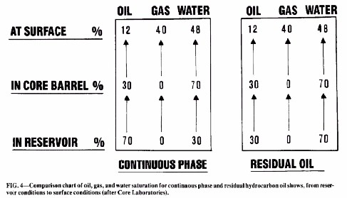
Figure 4. Comparison chart of oil, gas, and water saturation for continuous phase and residual hydrocarbon oil shows, from reservoir conditions to surface conditions (after Core Laboratories).
The exploration implication of the physical modes of hydrocarbon occurrence or show classification scheme are somewhat different from the production implications (Figure 1). Continuous phase shows in reservoir quality rock indicate a trapped accumulation of oil or gas. None of the other show types or modes of occurrence indicate a trapped accumulation. Residual shows indicate that liquid hydrocarbons migrated through the oil- or gas-stained rocks. Dissolved hydrocarbons indicate that hydrocarbons are present in molecular form in the system but do not demonstrate bulk oil or gas is present. Hydrocarbons in kerogen indicate only that liquid oil or gas is potentially available to the system in the form of a hydrocarbon source rock, but indicate nothing about the release migration or the entrapment of liquid-producible oil or gas.
Identification of Type I Shows
Exploration implications of each show type vary from direct indications that a trapped accumulation has been located, to the identification of potential source rock zones. Total ramifications of each show type are beyond the scope of this paper. However, from the standpoint of direct exploration application, the single most important show type is type I, continuous phase mode of occurrence, which indicates the discovery of a trapped accumulation of oil or gas of unknown size. Can type I shows be identified? What data are necessary to differentiate between migration paths (type II shows) and trapped accumulations (type I)?
Hydrocarbon shows in exploratory wells can be divided into shows seen directly in cuttings or cores, shows of oil or gas recovered during testing or in the drilling fluids, and shows inferred from wireline or gas detector logs. To examine how type I shows can be separated from type II, we must determine what data each hydrocarbon indication provides. A potential way of distinguishing between show types is to determine the percentage of pore space that must be occupied by oil or gas to positively identify a continuous phase model of occurrence, and then, the type of fluid recovery needed for a positive identification of a type I show.
A continuous phase show was defined as a slug or filament of oil or gas with a continuous connection through the pore network of the rock. The minimum hydrocarbon saturation necessary to establish a continuous filament through a porous rock is approximately 10% (Schowalter, 1979). The minimum saturation for a type I show then could be as low as 10%. Maximum saturations for type I shows could be as high as 90%, depending on the irreducible water saturation of the oil-saturated rock in question. The minimum saturation for a residual or droplet-scale type II show is about 5 to 10%, depending on the initial hydrocarbon saturation in the rock before water displacement (Figure 3). The average maximum saturation for water displacement residuals in sandstone reservoirs is 35%; in carbonate reservoirs, residual saturations can range from 30 to 60% and average 55%. Vuggy carbonates can have residual saturations in excess of 60% and can approach 80% in oomoldic porosity. Based on saturation of pore space, the only way to positively identify a type I continuous phase show would be to determine from cuttings, cores, or logs that the rock in question had a hydrocarbon saturation in excess of 35% for a sandstone reservoir or 55% for a carbonate reservoir.
What is the possibility of cuttings, core, or log data providing accurate hydrocarbon saturation data that can be used to distinguish between type I and type II shows? Because of the normal rotary drilling process, neither cuttings nor cores can provide useful information concerning subsurface hydrocarbon saturation. Safe drilling procedures require drilling fluid or mud column pressure to be greater than formation pressure, and water will be filtered from the drilling fluid into any permeable rocks penetrated by the drill bit. This filtration action is comparable to a waterflood process in reservoir rocks, and any mobile continuous phase oil or gas occurrence near the well bore will be reduced toward a water displacement residual saturation. Furthermore, as the rock core or cutting is moved to the surface, the reduced pressure environment at the surface causes gas to come out of solution and to expel additional liquid hydrocarbons and water from the rock pore space. Any data from cutting or core samples, therefore, would not indicate the true subsurface saturation and are useless in separating type I from type II shows, unless core saturations exceed 35% in a sandstone reservoir or 55% in a carbonate reservoir. This problem is very clearly illustrated by a Core Lab diagram (Figure 4), which shows that a residual subsurface saturation of 30% oil could have, by laboratory analysis, the same saturations of oil, gas, and water at the surface as a continuous phase subsurface oil saturation of 70%.
The exception to this rule would be in the case of low gravity, viscous oils with no associated gas. These types of oil may not be flushed from the reservoir during drilling and may reflect subsurface oil saturations on core analysis.
The one way to overcome the problem of core analysis not being representative of subsurface saturation is to stop the mud filtration process by pressure coring. Pressure coring can provide saturations at subsurface conditions, but is expensive and not routinely used.
By measuring reservoir porosity and resistivity, wireline logs can provide data on oil or gas saturation in the reservoir. Oil or gas saturations from logs are generally based on data obtained beyond the zone of mud filtration of flushing, and therefore, provide saturation data at subsurface conditions. Type I, continuous phase shows, then can be identified indirectly from log-calculated oil or gas saturations that are in excess of 35% for a sandstone reservoir or 55% for a carbonate reservoir. The reliability of these calculations and subsequent show classification will be a function of the quality of log data, depth of filtration, and accuracy of the measured or inferred formation water resistivity. Such log calculations are subject to error and must be weighted, based on experience in the area and trial and error. Recent logging advances that calculate the inferred presence of movable oil may also act as a positive indicator for type I shows. Residual, type II shows, by definition, have no movable oil because oil occurs as isolated unconnected droplets with no permeability to oil. In contrast, type I shows are connected filaments of oil or gas that would be movable upon being flooded by water from the mud filtration process during drilling. Movable oil correctly interpreted on logs then is a positive indication of a type I oil occurrence.
In general, hydrocarbon saturations of greater than 35% in sandstone and 55% in carbonates from cores or logs and movable oil from log calculations, can be considered as positive indicators of type I hydrocarbon shows. Oil-stained cuttings, cores, and log-calculated oil saturations less than 35% for sandstones and 55% for carbonates cannot be used to separate type I or type II shows.
A second potential method of distinguishing type I and type II shows is by analyzing the type and amount of fluid recovered from a reservoir zone that is oil stained during drilling or testing. From the standpoint of fluid recovery, the main difference between type I and type II shows is that type I shows have some relative permeability to oil and type II shows have no relative permeability to oil. By using this concept, any indication of the movement of oil from the rock into the well bore during testing or drilling would be a positive indication of a type I, continuous phase, subsurface show. In contrast to the problems in differentiating show types by calculated hydrocarbon saturation, the fluid recovery concept provides a direct way of identifying type I shows. Any significant recovery of free oil on drill-stem or production tests would positively identify a type I show. This indication of free oil could be in the form of oil-cut mud, oil-cut water, free oil, etc. Flecks or rainbows of oil in mud or water are not reliable indications of type I shows. The total amount of fluid and percentage of oil versus mud or water is important in determining if the oil show may be economic in the well bore being tested, but not in the identification of a type I show.
Minor amounts of oil-cut mud recovered during drilling are not a decisive indicator of type I shows because the grinding action of the bit may create oil-cut mud by releasing isolated drops of residual oil trapped in the rock-pore space. Significant volumes of oil while drilling (e.g., oil on the pits) can be considered a conclusive indication of a type I show, as the volume required to explain this type of show would be greater than the volume that could be liberated by drilling the cylindrical rock column penetrated by the bit.
Interpretations of gas shows while drilling or testing are more difficult than oil shows. Gas-cut mud observed while drilling and mud-logging shows can result from any of the four modes of occurrence. Gas can be liberated by the grinding action of the bit from gas adsorbed on rock grains, in coals, or in oil source rocks. Gas in solution in the pore water of subsurface rocks can produce gas-cut mud while drilling, which may be seen as mud-logging shows. The grinding action of the bit can liberate residual gas droplets in the pore space of reservoir rocks, which can also create gas-cut mud and mud-logging shows. Drilling continuous phase gas occurrences will also liberate gas from the rock pore space and create gas shows. Indications of gas while drilling cannot be used as an unequivocal indicator of type I shows. This is even true in high-pressure zones where mud weight must be increased to prevent gas blowouts, as this condition can be created by gas in solution as well as from gas in a reservoir.
Gas recovered during a formation test can result from three of the four types of subsurface gas occurrences: (a) continuous phase gas whereby gas inflow occurs during the test; (b) residual gas which expands due to a pressure drop at the well bore and forms a local continuous phase with subsequent gas inflow; and (c) gas dissolved in formation water whereby water inflow occurs and the contained gas exsolves owing to the pressure drop at the well bore.
Positive indicators for a continuous phase type I occurrence from formation testing would be gas coming to the surface at a sustained measurable rate. Residual gas and solution gas occurrences should not be able to produce a sustained free gas flow. An exception to this concept would be when a permeable water-bearing reservoir, saturated with gas in solution, flows to the surface. Continuous measurable amounts of gas could then be produced as a separate phase with the water. Gas-cut water or gas-cut mud during testing could indicate any of the three modes of occurrence listed above.
The first key question in interpreting hydrocarbon shows in exploratory wells is distinguishing between continuous phase type I and residual type II modes of occurrence. From the discussion, it is obvious that there are few absolute identifiers for type I continuous phase shows. Subsurface hydrocarbon saturation of greater than 35% for sandstone and 55% for carbonate from cores or logs is an indirect indication of a type I occurrence. Indications of movable oil from logs is also a positive indirect indicator of a type I show. For oil, any free oil recovery during formation testing or significant volumes of oil while drilling is an indication of a type I show. In the case of gas, a formation test of gas coming to the surface at a sustained measurable rate is an indication of a type I gas occurrence. If type I continuous phase shows can be positively identified in an exploratory well, a trap of unknown size has been identified. Even if the well bore where this show is located is evaluated as noncommercial, significant exploration information has been gained by drilling the test and interpreting the shows.
If a show has been identified as a type I show, it can be interpreted quantitatively to determine the size of the oil or gas column required to create the show. Producing oil or gas reservoirs are, by definition, continuous phase shows. As mentioned in the introduction, these shows can be used to estimate the oil or gas column required to force oil in the pores of a water saturated reservoir.
In order to validate this exploration technique, a controlled field study was attempted. In the field case history, the hydrocarbon shows in the reservoir zone of a producing well in Buffalo field, South Dakota, were interpreted quantitatively, and an estimate of the elevation of the oil-water contact was attempted and compared to the known oil-water contact in the field.
Extrapolation Case History--Buffalo Field
Buffalo field, Harding County, South Dakota, produces from the Ordovician Red River "B" zone at depths between 8,300 and 8,500 ft (2,530 and 2,590 m). This stratigraphic trap is located on the east flank of a faulted anticline (Figure 5). Dip is eastward across the field at about 1°. If the field is one continuous accumulation, the maximum vertical oil column in the field would be about 380 ft (116 m). The field, discovered in 1954, has produced 4 million bbl of oil and is still being developed.
The reservoir at Buffalo field is a sucrosic, vuggy dolomite. The main productive interval is 15 to 18 ft (4.6 to 5.5 m) thick, consisting of an algal, laminated boundstone to wackestone. Reservoir porosities range from 16 to 29% and apparent air permeabilities range from less than 1 md to 36 md. The reservoir is underlain by a vuggy lime wackestone with 4% porosity and permeabilities less than 0.01 md. The lateral seal for the accumulation appears to be a chalky-textured dolomitic limestone. The cap rock and seat seal for the trapped accumulation are bedded anhydrite and lithographic limestone.
Figure 5. Structural contour map on top of Ordovician Red River Formation "B" porosity, Buffalo field, Harding County, South Dakota.
The boundaries of Buffalo field are not yet clearly defined. Wells updip from the field commonly test oil at noncommercial rates, suggesting a gradual facies change from commercial reservoir to the updip lateral seal. The trapping edge can be mapped regionally by a thinning of the Red River "B" zone from a maximum of 20 ft (6 m) in Buffalo field to zero west of the field. The downdip limits of the field are also poorly defined; production extends downdip to approximately the -5,600 ft contour (Figure 5). Downdip, the Red River "B" tests mainly water, suggesting an oil-water contact at approximately -5,600 ft (-1,706 m).
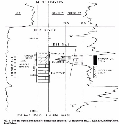
As a test case of estimating the oil column downdip from a commercially productive well, a cored well from Buffalo field was studied and the shows in the reservoir zone were interpreted quantitatively. The well used in the study was the Kirkwood 14-31 Travers, located in Sec. 31, T21N, R4E, Harding County, South Dakota (Figure 6). The well was drilled in 1978 and completed pumping from the Red River "B" zone at a rate of 180 bbl of oil per day and 150 bbl of water per day. The well was completed in June 1978 and had produced 70,764 bbl of oil as of January 1981, with reservoir estimates of more than 200,000 bbl of recoverable oil. The 14-31 well was cored between 8,358 and 8,515 ft (2,547.5 and 2,595 m). The core description and log response for the Upper Red River interval are illustrated in Figure 6.
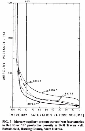
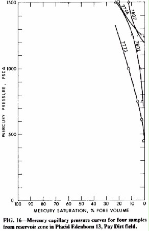
The Red River "B" reservoir in the 14-31 core is sucrosic, vuggy dolomite that is uniformly oil-stained throughout. Four samples from the pay section were tested in the laboratory to determine their capillary pressure properties (Figure 7). Log calculations for the "B" zone indicate an average water saturation of 20% and a corresponding oil saturation of 80%. As in most log calculations, this saturation value represents an average saturation through the best 8 to 10 ft (2.4 to 3 m) of the "B" reservoir. The shows in each sample were quantitatively interpreted by determining the mercury pressure required to explain an 80% mercury saturation of the pore space. The mercury pressure was then related to the oil column required to buoyantly produce the same oil saturation in the sample in the subsurface (Schowalter, 1979).
Figure 6. Core and log data from Red River Formation in Kirkwood 14-31 Travers well, Sec. 31, T21N, R3E, Harding County, South Dakota.
The assumptions used in the calculations were: (1) reservoir displacement pressure at 10% saturation of 40 psi mercury (Figure 7), based on the displacement pressure of the best reservoir rock tested; (2) subsurface oil-water interfacial tension of a 20.4 dynes/cm, based on a laboratory measurement of a crude oil sample from the field and a simulated water sample at a temperature of 180°F (this subsurface interfacial tension value results in a conversion factor of 0.055); (3) subsurface water density of 1.01 g/cc, based on a salinity of 18,000 ppm; (4) subsurface oil density of 0.837 g/cc, based on a 32° API gravity oil with a gas-oil ratio of 100; (5) water-wet rocks; (6) hydrostatic conditions; (7) mercury interfacial tension of 480 dynes/cm; (8) mercury-air-solid contact angle of 40°.
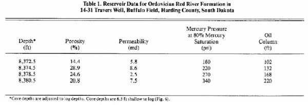
The results of these calculations are listed on Table 1. As mentioned previously, the calculations are based on an 80% oil saturation for each sample, based on log calculations averaged through a 10-ft (3 m) interval. Log calculations for each individual sample were not attempted because of the inaccuracies that would be involved in trying to correlate a 1-ft (0.3 m) zone in the core to correlative log values, and the averaging effect inherent in the log values because of tool spacing. The 80% oil saturation for the pay interval seems to correlate with the fluids actually produced from that zone. After 1 year, this well was producing oil at a rate of 100 bbl/day with 17 bbl water. Inspection of a typical relative permeability curve (Figure 2) suggests that a rock with an 80% oil saturation should produce 80 to 100% oil and 0 to 20% water.
As calculated from the four samples tested, buoyancy pressure required to force oil into 80% of the pores indicates an oil column in the range of 102 to 220 ft (31 to 67 m) and averaging 155 ft (47 m). If Buffalo field is one continuous oil column, the maximum oil column downdip from the 14-31 Travers well is approximately 330 ft (100 m) (Figure 5). Interpretation of the data from these four samples suggests that a minimum oil column on the order of 102 ft (31 m) should be present downdip from the analyzed well and that an oil column of up to 220 ft (67 m) may be present. The calculations suggest that a large oil column, up to 220 ft (67 m), is present downdip from the 14-31 well. This value is less than the inferred oil column from subsurface studies of 325 ft (99 m) and may indicate that Buffalo field is a complex trap consisting of two separate accumulations.
Figure 7. Mercury capillary pressure curves from four samples in Red River "B" productive porosity in 14-31 Travers well, Buffalo field, Harding County, South Dakota.
Table 1. Reservoir Data for Ordovician Red River Formation in 14-31 Travers Well, Buffalo Field, Harding County, South Dakota
If the 14-31 well had been the discovery well and if the outlined procedure had been followed, the resulting information could have been valuable in defining the limits of Buffalo field. The large oil column calculated would have allowed wells to be drilled downdip as much as 220 ft (67 m) and would have spurred field development. The estimated downdip limits of the field can be adjusted with the addition of information from subsequent wells.
Application of these principles could be used in developing newly discovered fields. If the calculated oil column is significantly larger than the mapped structural or stratigraphic closure for the prospect, additional wells should be drilled downdip to establish the field limits. If the calculated oil column is significantly less than the predicted oil-water contact from structural or stratigraphic closure, the prospect may be only partially filled and downdip development dry holes could be avoided.
The Buffalo field example suggests that the quantitative interpretation of type I, continuous phase shows, can be potentially quite useful in field development by estimating the oil-water or gas-water contact in the field from one well bore. The same approach is potentially applicable to quantitative interpretation of type I shows from wells that are not commercial producers.
If a type I show has been identified in a noncommercial reservoir, a trapped accumulation of oil has been located. The downdip oil or gas column associated with the identified type I show can be calculated in an analogous fashion to the producing well example. This concept would be very useful in an exploration setting where the show could be used as quantitative proximity indicators to hydrocarbon accumulations.
Before noncommercial type I shows can be interpreted, a model for the complexities of oil-water and gas distribution in stratigraphic traps must be developed.
EXPLORATION OF TYPE I SHOWS IN COMPLEX STRATIGRAPHIC TRAPS
Simple Stratigraphic Trap Model
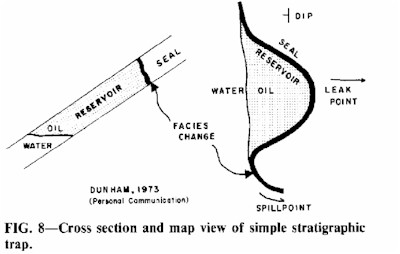
Figure 8 illustrates a simplified model for a stratigraphic trap, which is used by many explorationists. The model consists of a reservoir bed overlain and underlain by sealing shales. The reservoir terminates updip by a lateral facies change into an impermeable shale, and the geometry in map view of this lateral facies change is convex updip, forming a classic stratigraphic trap. In the model, the facies change from reservoir to updip lateral seal is assumed to be abrupt and obvious. In the downdip direction, the change from oil-bearing reservoir to water-bearing reservoir is assumed to be abrupt with no significant oil-water transition zone. Exploration efforts to explore for the above-described model are focused on mapping the geometry of the reservoir-seal boundary.
Once a stratigraphic prospect has been defined by various exploration methods, a drilling program is planned to attempt to discover the inferred stratigraphic trap. It is assumed that a well will be drilled either in or out of the field. Wells drilled within the inferred oil field are generally assumed to be easy to recognize. Wells that miss the economic part of the trap are assumed to be drilled in the seal facies or in water-saturated reservoir rock. Subsequent wells can then be located downdip from a seal facies or updip from the water-wet reservoir until the accumulation is located.
Complex Stratigraphic Trap Model
In a simple stratigraphic trap model, the boundary of the oil reservoir is sharp and clearly defined. Updip from the oil-bearing reservoir, reservoir-quality rock changes abruptly to the updip seal. Downdip, the oil-bearing reservoir rock changes abruptly to water-saturated reservoir-quality rock with no oil shows. An abrupt change from reservoir rock to the updip lateral seal occurs in many stratigraphic traps and has been confirmed frequently by drilling. However, development drilling of numerous other stratigraphic fields has revealed a gradual change updip from economic reservoir, to noneconomic oil-stained rocks, to a seal with no oil shows.
Abrupt downdip changes from oil-productive reservoir to rocks that produce all water, forming sharp oil-water contacts, occur in some oil fields. However, case histories show that in many other fields the downdip change from primarily oil production to 100% water production may be quite gradual and occur over a significant vertical distance (Aufricht and Koepf, 1957). This gradual change downward through a zone of mixed oil and water production to the downdip limits of an accumulation is called the oil-water transition zone by reservoir engineers. The width of this zone is controlled primarily by the average pore size and pore-size distribution of the reservoir rock. Reservoir rocks with pore systems consisting of large, connected, uniformly sized pores will have almost no oil-water transition zone. Reservoir rocks with a heterogeneous distribution of pore sizes and primarily small pores can have very thick oil-water transition zone. The thickness of any oil-water transition zone can be estimated if reservoir capillary properties and relative permeability are known (Arps, 1964; Schowalter, 1979).
Figure 8. Cross section and map view of simple stratigraphic trap.
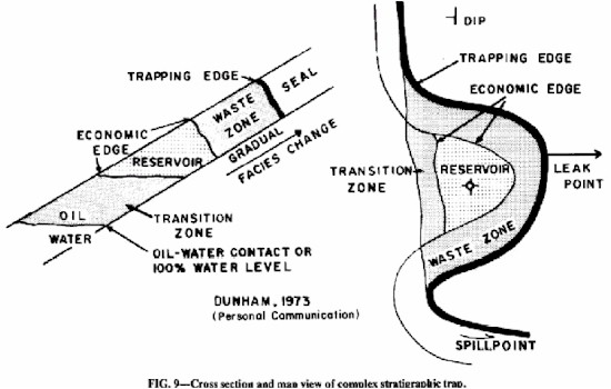
This simple stratigraphic trap model must then be modified to accommodate a facies change from reservoir to seal in the updip direction and from oil-productive to water-productive reservoir in the downdip direction. A more complex stratigraphic trap model is illustrated in Figure 9 and Figure 10. This model shows an oil-productive reservoir that changes gradually updip from reservoir rock to oil-stained noncommercial rocks. The seal is called the "trapping edge" of the accumulation. The boundary between the economically producible, oil-saturated reservoir rock and the noneconomic oil-stained rock is called the "economic edge" of the accumulation. The area between the trapping edge and economic edge of a stratigraphic trap is termed the "waste zone" (Dunham, personal commun.). The term "waste zone" is used because the oil and/or gas cannot be produced economically and is therefore wasted. Definition of the waste zone is based on economics, and of course will vary from area to area.
The model also shows a gradual transition downdip from water-free oil production in the economic reservoir to downdip water production. This zone between the water-free oil-productive reservoir and the downdip water-productive reservoir rock is termed the "oil-water transition zone." Both transition zone and waste zone are economic terms that can vary in identical reservoirs if depth or other factors significantly affect the economics of production. The width and thickness of the oil-water transition zone will depend on the pore sizes and pore-size distribution in the reservoir rock and the physical properties of the oil and water in the reservoir (Arps, 1964).
The complex model has three zones in which shows will be seen: (1) the oil-water transition zone, (2) the economic reservoir, and (3) the waste zone. Two of the three zones in such traps will not be economic. Depending on the width of the transition zone and the waste zone, the odds of drilling into the uneconomic portions of a trapped oil accumulation may be greater than drilling into the economic area of the trap. Where this type of complex trap is encountered, then it is vital to identify where a type I show occurs in the complex model.
It can also be demonstrated that if the transition and waste zones are thicker than the total oil column that can be trapped by a given seal facies or trap geometry, there may be no economic reservoir. The oil column trapped in any stratigraphic accumulation will depend on the geometry of the facies change (spillpoint) and the lateral seal capacity of the updip trapping facies (leak point). The width of the waste zone will depend on the abruptness of change in facies from reservoir to seal. The stratigraphic explorationist then must be able to recognize the waste zone and the oil-water transition. What are the characteristics of these zones?
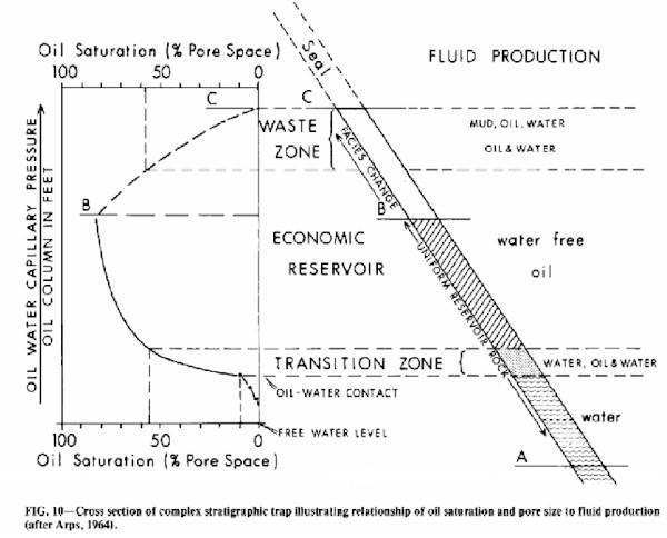
To compare and contrast these two zones, further analysis of the complex stratigraphic trap model is necessary. Figure 10 shows a cross section of the complex model. In this diagram, the reservoir from point A to point B is assumed to be uniform and homogeneous. This means that the pore size and the pore-size distribution within the reservoir are the same at any point from A to B, and if capillary pressure curves were run on multiple reservoir rock samples between points A and B, the capillary pressure curves would be identical for all samples. For a completely uniform reservoir as illustrated, the oil saturation in the reservoir would gradually increase above the 100% water level as buoyant pressure in the oil column increases (Schowalter, 1979). The buoyant pressure would be equivalent to the capillary pressure of the oil and water in the rock at any saturation. The solid line in the capillary pressure diagram then can be considered the capillary pressure curve for the uniform reservoir at any point from A to B, and the oil saturation in the reservoir at any point between the 100% water level point B in the model.
Figure 9. Cross section and map view of complex stratigraphic trap.
From point B to point C, the reservoir zone gradually changes facies and becomes a rock with pores small enough to seal the accumulation. This facies change is assumed to be a linear reduction in pore size from point B to C. Capillary pressure curves from rock samples along line BC would all be different. The gradual reduction in pore size in the reservoir zone would gradually decrease the oil saturation in the reservoir zone from point B to C, as shown by the dashed line on the capillary pressure diagram. The oil saturation would become zero at the trapping edge of this facies change (Figure 10). This change in pore size could occur without a decrease in porosity from B to C.
Transition Zone Characteristics
By analysis of Figure 10, we can discuss the potential differences between the waste zone and the oil-water transition zone. The type of fluid they produce is one way of differentiating these zones. The oil saturation through the transition zone generally ranges from 10% to between 50 to 60% of the reservoir pore volume. From inspection of typical oil-water relative permeability curves (Figure 2), the minimum oil saturation needed to have any permeability to oil can be as high as 20%. Toward the base of the oil-water transition, a fluid production test of oil-stained rocks in a trapped accumulation could produce 100% water. As the oil saturation in the reservoir zone increases above some minimum level, the transition zone can produce oil and water in varied percentages up to the top of the transition zone where the reservoir would test 100% oil. The transition zone can then produce all water or some combination of oil and water. Formation tests in the transition zone should yield fluid at high rates because, by definition, the reservoir zone is generally uniform from the oil-productive reservoir through the transition zone into the water-productive reservoir. High fluid-productivity rates from oil-stained rocks may be indicative of an oil-water transition. Oil saturation in a transition zone may vary in the model from a high of 50% to a low of 10%. Oil saturations less than 50% in reservoir-quality rock probably indicate an oil-water transition zone. Any nonreservoir rocks with smaller pores and correspondingly higher capillary pressures should be water saturated and have no visible oil stain in cores or other samples. Toward the base of an oil-water transition zone, very slight changes in pore sizes or capillary properties of the rocks may cause erratic distribution of oil staining. Vertical change of oil-stain pattern, in what appears to be uniform reservoir-quality rock, would be an indicator of an oil-water transition zone. Oil saturations can be related to the oil column required to create the saturation, if the capillary properties or pore sizes of the oil-stained sample can be determined. Calculations of oil shows in the transition zone should suggest small columns. The oil column required to explain a low oil saturation in a reservoir-quality rock should be on the order of 10 to 20 ft (3 to 6 m), as the minimum oil column required to migrate through an average reservoir is on the order of 10 ft (3 m). Calculations of oil columns required to explain oil saturation in an unstained rock and adjacent to oil-stained reservoir rocks should also suggest small oil columns and be indicative of an oil-water transition zone.
Figure 10. Cross section of complex stratigraphic trap illustrating relationship of oil saturation and pore size to fluid production (after Arps, 1964).
In Figure 10, pore size decreases from point B to C. Above point B, the reservoir will continue to have water-free production until the oil saturation is reduced sufficiently to cause some relative permeability to water. From the base of the waste zone to the seal, the oil saturation will gradually decrease from 50% to zero. Based on inspection of typical relative permeability curves (Figure 2), the waste zone with oil saturation from 50% to zero could produce both oil and water during a fluid-production test. As the oil saturation in the waste zone is reduced to around 20%, the waste zone could produce only water from oil-stained rocks. If the waste zone is low permeability rock that has its permeability further damaged while drilling, it may produce only mud or oil-cut mud. The waste zone, based on the model, can yield, at different times mud, oil, oil and water, and 100% water.
The waste zone can produce the same type of fluid as the oil-water transition zone. The type of fluid produced from an oil-stained rock is not diagnostic in determining if an oil show is in a waste zone or a transition zone. Conventional exploration wisdom for stratigraphic traps suggests moving updip from oil-stained rocks that produce water or oil and water. This may be incorrect, as both a waste zone and a transition zone may produce the same type of fluids. How can we distinguish between the waste zone and the transition zone if the type of fluids produced can be the same?
As defined in the complex model, the pore size of the reservoir bed decreases from the reservoir to the seal. As pore size is reduced, permeability is reduced and the waste zone should not be able to produce any fluid at economic rates. Fluid productivities in waste zones should be low.
Calculations of oil column based on oil saturations and rock capillary properties in the waste zone should indicate a large vertical oil column. Within the waste zone, any thin interbedded reservoir-quality rocks should be oil stained and have high oil saturations. Nonreservoir quality rocks or "tight" rocks in the waste zone may be oil stained. This contrasts with the transition zone where nonreservoir quality or "tight" rocks should not be oil stained.
Exploration Implications of Transition and Waste Zones
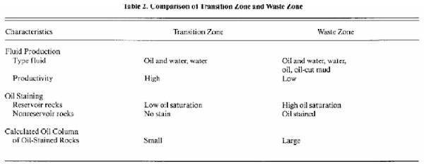
The characteristics of the waste zone and the transition zone are summarized in Table 2. These two zones cannot be distinguished reliably by the type of fluid they produce. They can be differentiated by fluid productivity, the type of rocks that are oil-stained, and the calculated oil columns required to explain oil shows in cores or samples. Based on an analysis of the complex model, it appears that sufficient differences exist between waste zones and oil-water transition zones to allow them to be distinguished. Data generally available from exploratory wells should allow one to relate oil shows in "tight" rocks to the complex stratigraphic model.
Table 2. Comparison of Transition Zone and Waste Zone
If oil-stained samples can be identified as being in the oil-water transition, the operator should drill updip from the oil shows. The amount of structural elevation gain needed to move out of the oil-water transition zone into water-free oil production can be quantified if the capillary properties of the reservoir and the oil saturation of the location of the first test well are known (Arps, 1964; Schowalter, 1979).
If oil shows can be determined to be in the updip waste zone of a stratigraphic trap, the total oil column downdip in the trapped accumulation can be calculated. If a large oil column is calculated, the operator may have discovered an oil accumulation or trap of significant extent. If reservoir quality rocks can be predicted to occur downdip from the waste zone well, additional wells are justified downdip of the first test to locate the economic portion of the discovered field.
SHOW INTERPRETATION-EXTRAPOLATION CASE HISTORIES
If oil or gas shows can be classified as type I, continuous phase shows, and placed in the complex stratigraphic trap model, exploration efforts can be guided by interpretations of hydrocarbon show data. What is the likelihood of classifying shows as to their mode of occurrence? If a show is classified as a type I continuous phase mode of occurrence, how can this show information be used to interpret the show in a complex stratigraphic model? If well shows indicate a waste zone has been penetrated, how accurately can the oil or gas shows be related to the trapped hydrocarbon column? Can shows be characterized as being in the oil-water transition zone, and be quantitatively interpreted?
To attempt to answer these questions, four complex stratigraphic traps were studied. For the sake of brevity representative field studies of a waste zone well and a transition zone well will be documented. The geologic and geographic identifiers for each field have been removed from each case history at the request of Shell Oil Co.
Figure 11. Structure contour and fluid production map of Pay Dirt field.
Pay Dirt Field--Gas Waste Zone
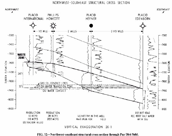
Pay Dirt field is a stratigraphic trap that produces oil and gas from a biohermal reef buildup located along a regional northeast-southwest-trending shelf edge. The trap at Pay Dirt field is caused by a facies change crossing a slight structural nose (Figure 11). The facies change is from porous and permeable reef rock to fine-grained rock of lagoonal-origin and high displacement pressure. The present-day structural nose was formed by regional tilting to the southeast of a curved organic reef buildup that extended out from the shelf-edge barrier into a lagoon to the northwest. Lithologies of the lateral seal are gray lime mudstone, wackestones, and black calcareous shales and lime mudstones. The trapped vertical hydrocarbon column at Pay Dirt field is greater than 280 ft (85 m), consisting of a 35-ft (10 m) oil column and a gas column greater than 245 ft (75 m; Figure 12). Regional dip is 120 ft/mile to the southeast with no mappable faulting in the field area. Pay Dirt field produces from 38 oil wells and 7 gas-condensate wells, with a probable ultimate recovery of 120 million bbl of liquid hydrocarbons plus 670 bcf of gas.
Based on distribution of the reservoir facies, lateral seal facies, and shows (Figure 11), it is inferred that the size of this stratigraphic accumulation is controlled by trap geometry, and oil and gas have spilled updip to the north. The field limits do not appear to be controlled by the lateral seal capacity of the updip lateral seal.
The reservoir rock at Pay Dirt field is a vuggy lime packstone to boundstone facies. The rock matrix is chalky lime mudstone, with the amount of matrix porosity depending on intergranular cement. Scattered oolitic porosity interbedded with calcareous shales is present along the western edge of the reservoir. The most productive porosity is vugular, with vugs ranging from pinpoint to 1.5 in. (3.8 cm). Porosities for the reservoir average 16% and permeabilities average 108 md; the cut-off porosity for production is approximately 8%. The main reef-building fossils are rudistids, other pelecypods, gastropods, and stromatoporoids. The environment of deposition is interpreted to be a curved back-reef organic buildup that extended off a linear shelf-edge barrier reef into a lagoon. Reservoir porosity is present downdip from the field and the top of the oil-water transition zone is placed at -7,870 ft (-2,399 m; Figure 11, Figure 12). Oil shows are present below this level, indicating that the actual oil-water contact, or 100% water level, is somewhere below this point.
Figure 12. Northwest-southeast structural cross section through Pay Dirt field.
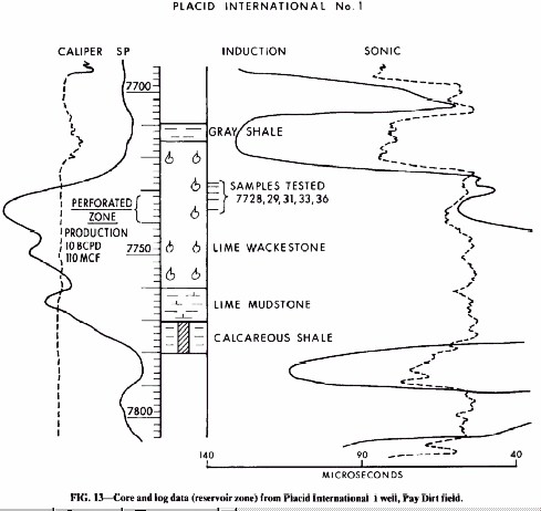
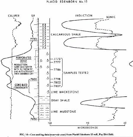
Immediately updip from commercial production at Pay Dirt field, there are two noneconomic gas wells and three other wells with gas and oil shows (Figure 11). Two of these wells, Placid International 1 and Placid Edenborn 13 (Figure 11) cored the reservoir-equivalent horizon; they were sampled and studied as waste zone wells to determine if the gas column downdip could be accurately calculated from core data. The more porous and permeable samples, based on visual observation, were selected for study from core chips obtained from the original whole core. Samples were collected from well 1 in and just above a zone that was completed at 10 bbl/day oil and 110 mcf gas (Figure 13). Samples were collected from a perforated zone in well 13 from which acid water with shows of gas and condensate were swabbed: the zone then was swabbed dry (Figure 14). Samples were also taken from well 13 in a section of core that bled condensate (Figure 14).
The gas show in well 1 was interpreted to be a type I continuous phase show, because gas was recovered at a measurable rate from the reservoir zone during a production test. Well 13 recovered acid water with a show of gas and condensate during production tests, and the core from a lower zone bled condensate. Well 13 is also tentatively classified as a type I occurrence because of these shows, even though it did not flow gas at a sustained rate.
In this discussion, shows in wells 1 and 13 are interpreted to be continuous phase gas occurrences directly associated with a trapped gas accumulation. As these type I shows are found in rocks of low permeability that will not produce at economic rates, they are considered to be in the waste zone of a complex stratigraphic trap. This inference from the well data in wells 1 and 13 is substantiated by drilling results from Pay Dirt field and vicinity (Figure 11).
Figure 13. Core and log data (reservoir zone) from Placid International 1 well, Pay Dirt field.
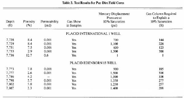
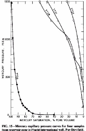
Core samples from the apparently gas-saturated intervals in these two wells were analyzed in the laboratory for porosity, permeability, and mercury capillary pressure (Table 3). Mercury displacement pressures were recorded at 10% pore volume saturation of the capillary pressure curves (Figure 15, Figure 16) and are listed in Table 3.
Each sample was examined by standard show examination techniques (Swanson, 1981). No shows were observed, but this is not unexpected, as gas shows in samples are generally difficult to detect. The gas saturation in the pore space of each sample in the subsurface could not be accurately calculated from logs. When hydrocarbon saturations of the pore space of an oil- or gas-saturated rock cannot be made because of low porosity or too thin a bed, oil or gas column estimates can still be calculated. The technique is to calculate the minimum vertical oil or gas column required to produce a 10% pore space saturation which is the minimum saturation needed to produce a continuous phase show. The gas column calculation required to produce a 10% saturation is listed in Table 3 for each rock sampled and are based on the following assumptions: (1) displacement pressure of reservoir was assumed to be zero, because the reservoir is vuggy carbonate, with vugs up to 1.5 in. (3.8 cm), which should have a very low displacement pressure; (2) a subsurface gas-water interfacial tension of 30 dynes/cm (Schowalter, 1979) (this interfacial tension value results in gas-water conversion factor of 0.08); (3) subsurface water density of 1.09 g/cc, based on a salinity of 100,000 ppm; (4) subsurface gas density of 0.18 g/cc, based on a surface specific gravity to air of 0.713, extrapolated to reservoir temperature and pressure (Schowalter, 1979); (5) water-wet rocks; (6) hydrostatic conditions, based on study of the potentiometric surface of the reservoir zone; (7) mercury interfacial tension of 480 dynes/cm; (8) mercury-air-solid contact angle of 40°.
Figure 14. Core and log data (reservoir zone) from Placid Edenborn 13 well, Pay Dirt field.
Most samples tested in both wells are lime wackestones with a very fine chalky texture. These rocks have porosities ranging from 2.6 to 8.4%, and apparent air permeabilities of less than 0.0001 md. Mercury displacement pressures, recorded at 10% pore volume saturation, ranged from 600 to 1,500 psi. Gas columns at 10% saturation were calculated and ranged from 123 to 300 ft (37 to 91 m) of vertical gas column.
The exception to the samples discussed is a vuggy lime packstone with a porosity of 12.7%, an apparent air permeability of 0.6 md, and a mercury displacement pressure of 1 psi. This sample, 7,736 (samples refer to depth in feet), is from the Placid International 1 and must account for the measurable production rates observed in this well.
Interpretation of the minimum gas column associated with these samples is difficult because the specific samples that were saturated with gas cannot be determined by show sample examination techniques in the laboratory. Samples 7,731 and 7,733 from well 1 are within the perforated zone that produces gas and condensate at a measurable but uneconomic rate. The vertical gas column needed to force gas into these samples is 123 ft (37 m) for 7,731 and greater than 300 ft (91 m) for 7,733. If sample 7,731 is actually saturated with gas in the subsurface, the minimum gas column associated with this sample is 123 ft (37 m); for sample 7,733 it would be greater than 300 ft (91 m). Sample 7,736 from the same well has a very low displacement pressure, and it is difficult to estimate the gas column associated with it, lacking an accurate subsurface gas saturation calculation from logs.
Samples 7,773 and 7,777 from well 13 are from a perforated zone that swabbed acid water with a show of gas and condensate (Figure 14). If either of these samples were saturated with gas in the subsurface, the minimum vertical gas column associated with these shows would be 185 ft (56 m) for 7,773 and greater than 300 ft (91 m) for 7,777 (Table 3). Samples 7,798, 7,802, and 7,807 are from the section of core in well 13 that bled condensate. If any of the tested samples bled condensate, and therefore were saturated with gas in the subsurface, the minimum vertical gas column associated with the show in these samples would be 257 ft (78 m; Table 3).
The problem of interpreting the results in these two wells is that, without well-site observations, it is impossible to determine which of the samples tested were actually saturated with gas in the subsurface. This problem could be eliminated in a wildcat well if careful core examination at the well-site enabled one to distinguish between core pieces that had shows of gas (e.g., bled gas or condensate) from those that did not.
The direct association of the samples tested with gas and condensate shows reported by core analysis suggests that most of the samples were saturated with gas in the subsurface. If the highest displacement pressure rock in each well is assumed to be gas saturated, the minimum gas column required to explain these shows would be approximately 300 ft (91 m). If all calculated gas columns are averaged, the estimated gas column is 242 ft (74 m). The gas column known to exist in the field is 245 ft (75 m), with an oil column below that of 35 ft (11 m). The 35-ft (11 m) oil column would create a buoyant pressure equivalent to approximately 15 ft (4.6 m) of additional gas column at the waste zone wells. The 242-ft (74 m) hydrocarbon column calculated as a result of the waste zone core study in Pay Dirt field correlated well with the actual gas equivalent column of 260 ft (79 m) known to exist in Pay Dirt field. Even more exact estimates might have been possible if detailed core descriptions had been available to determine which samples had gas shows and which did not. However, the average value for all samples thought to be gas saturated agrees very well with the gas column known to exist in the field.
Table 3. Test Results for Pay Dirt Field Cores
A large gas column is indicated by analysis of the data from these two wells. If either of these two wells had been drilled as wildcats, the procedure outlined here could be followed as an exploration technique. The interpretation would be that the shows in these wells are in the "waste zone" of a trap with a large gas column. Further exploratory wells could be drilled as much as 240 ft (73 m) lower, if there is any possibility of reservoir-quality rock within the laterally equivalent zone of the gas-saturated samples. The presence of the vuggy lime packstone (sample 7,736, well 1) would suggest that some reservoir-quality rock is present in the area, and if the vuggy lime packstone thickens downdip, commercial production should exist.
The approach to evaluating shows in oil-water transition zones is analogous to the approach used in the previous waste-zone example.
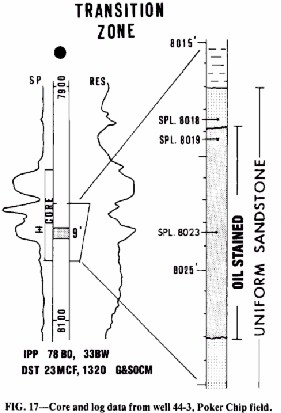
A transition zone was studied in well 44-3, Poker Chip field, a stratigraphic trap in a clastic sandstone-shale sequence at a depth of 8,000 ft (2,438 m). Logs and core information on the 44-3 well are illustrated on Figure 17. This well was cored from 7,071 to 8,047 ft (2,155 to 2,453 m). The lowest sand in the well was oil stained from 8,019 to 8,028 ft (2,444 to 2,447 m). A drill-stem test of the oil-stained interval flowed 23 mcf of gas per day, and recovered 1,320 ft of gas and slightly oil-cut mud. The well was selectively perforated in the oil-stained zone and was completed pumping 78 bbl of oil and 33 bbl of water per day. The well produced a total of 22,389 barrels of oil, 290 mcf gas, and 10,000 bbl of water over a 3-year period before being plugged and abandoned.
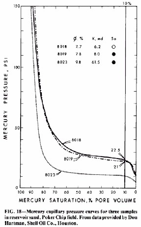
Quantitative core studies of the shows in the 44-3 well were undertaken as an example of a possible transition zone well. Careful examination of the core (Figure 17) shows that the upper contact of the oil-stained zone is sharp and appears to occur in a continuous uniform sandstone section with no observable lithologic break present at the oil-stain contact. Sample 8,018 was not oil stained and had a porosity of 7.7% and an apparent air permeability of 6.2 md. Sample 8,019 is oil stained and has a porosity of 7.8% and permeability of 8.0 md. The best foot of reservoir-quality rock in the oil-stained section of the core is sample 8,023 with a porosity of 9.8% and a permeability of 61.5 md. To interpret quantitatively the oil-stained core in this well, samples from just above the oil-stained zone (8,018), just below the oil-stain contact (8,019), and the best foot of reservoir (8,023) were tested in the laboratory to determine their mercury capillary pressure characteristics.
Figure 15. Mercury capillary pressure curves for four samples from reservoir zone in Placid International well, Pay Dirt field.
Figure 16. Mercury capillary pressure curves for four samples from reservoir zone in Placid Edenborn 13, Pay Dirt field.
The mercury capillary pressure curves for these samples are illustrated on Figure 18. Samples 8,019 and 8,023 were oil stained, sample 8,018 was not oil stained. Calculations of foot by foot oil saturations (such as sample 8,019 and 8,023) cannot be done accurately from logs because of the averaging of resistivity values due to tool spacing. The pressure required to create a 10% mercury saturation of the pore space of each sample was read off the capillary pressure curves and used to estimate minimum oil columns at a 10% saturation. Sample 8,018 had a 10% displacement pressure of 22.5 psi; 8,019, 21.0 psi; 8,023, 9.0 psi. The minimum oil column required to explain a 10% saturation in each sample was calculated, using the following assumptions: (1) minimum reservoir displacement pressure of 9.0 psi mercury, based on sample 8,023; (2) oil-water interfacial tension of 80 dynes/cm (this is an estimated value, as oil and water samples could not be obtained for actual measurements, and results in an oil-water conversion factor of 0.08); (3) subsurface water density of 1.01 g/cc; (4) subsurface oil density of 0.75 g/cc; (5) water-wet rocks; (6) hydrostatic conditions; (7) mercury-air interfacial tension of 480 dynes/cm; and (8) mercury-air-solid contact angle of 40°.
Based on the calculations, sample 8,018 would require a 10-ft (3 m) oil column to have a 10% saturation; sample 8,019 would require a 9-ft (2.7 m) oil column. The thickness of the oil-stained interval is approximately 9 ft (2.7 m).
Interpretation of these data suggests that the maximum oil column that could be present below sample 8,018 is approximately 9 ft (2.7 m). If an oil column greater than that were present, sample 8,018 should be oil stained, as there are no lithologic breaks between the samples to seal off the buoyant pressure acting on this sample. As the maximum oil-stained interval in the well is approximately 9 ft (2.7 m) and a 10-ft (3 m) column would be required to create an oil stain in sample 8,018, it would appear that the bottom of the oil-stained zone would be the oil-water contact for the accumulation at Poker Chip field. Quantitative show interpretation suggests that this well is probably in the oil-water transition zone of an accumulation and that no wells should be drilled down-dip from this well. Based on the drill-stem test and initial production from this well, it is not obvious that this well was a transition-zone well. Downdip wells could have been drilled unnecessarily without quantitative show interpretation.
Figure 17. Core and log data from well 44-3, Poker Chip field.
Figure 18. Mercury capillary pressure curves for three samples in reservoir sand, Poker Chip field. From data provided by Don Hartman, Shell Oil Co., Houston.
As in the previous case histories, the oil distribution in the rocks studied in the 44-3 well appear to be explainable by quantitative show interpretation techniques. If this well had been drilled as a wildcat, quantitative show interpretation could identify it as a transition zone well and strongly suggest that no downdip wells would be warranted, as they would be below the oil-water contact for the accumulation. The method used in this study was to compare capillary properties of oil-stained and non-oil-stained samples across an oil-stain contact. As seen in this sample, very slight changes in rock properties can control oil and water distribution in a reservoir. This change of oil stain across an apparently uniform interval of reservoir type rock is a good qualitative identifier of a transition zone. As illustrated here, oil shows can be qualitatively interpreted on location as cores are pulled and can be used in evaluation of the potential productivity of any oil-stained interval. More detailed quantitative studies can be made at a later date from the core samples to aid in choosing field development locations at the downdip edge of the field.
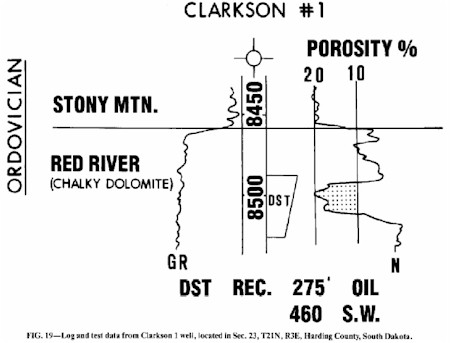
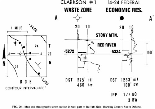
To illustrate the principles of hydrocarbon show classification and quantitative show interpretations in the framework of the complex stratigraphic trap model, a test case is used. The test well is the Clarkson 1, SW ¼ SE ¼, Sec. 23, T21N, R3E, Harding County, South Dakota (Figure 19). It was drilled to a depth of 8,526 ft (2,599 m) into the Ordovician Red River Formation. Oil shows were reported in samples from the Red River "B" zone from 8,492 to 8,512 ft (2,588 to 2,594 m). From a neutron porosity log, porosities in the "B" zone range from 17 to 20%. Based on sample shows while drilling, the zone was drill-stem tested and recovered 275 ft (84 m) of oil and 460 ft (140 m) of saltwater. The zone was retested and recovered 270 ft (82 m) of oil and 594 ft (181 m) of salt water. Based on the two drill-stem tests, it would appear that this well would produce oil, but with a high water cut (60 to 70%). The high water cut and fairly low total fluid recovery were used in evaluating the well as noncommercial, and it was plugged and abandoned.
What is the significance of this show of free oil? What are the exploration implications of this hydrocarbon show? The first step in show evaluation is to classify the hydrocarbon show as to its mode of occurrence. The Red River "B" zone drill-stem test produced free oil and was therefore classified as a type I continuous phase show. A type I show documents that a trapped accumulation of oil of unknown size had been located. If a trapped oil accumulation has been discovered, what are the limits, both economic and noneconomic, of the accumulation and what exploration implications can be drawn from these data?
Figure 19. Log and test data from Clarkson 1 well, located in Sec. 23, T21N, R3E, Harding County, South Dakota.
Cursory interpretation might place this oil show with high water cut in the transition zone of a trapped oil accumulation and might suggest a follow-up well be drilled updip to locate commercial oil production. This appears reasonable as the oil-stained zone has porosities up to 20%, and recovery of 864 ft (263 m) of total fluid on a drill-stem test indicates some reservoir permeability.
However, based on the concept that this well is a waste zone well and not a transition zone well, a well was drilled downdip. The 14-24 Federal well located in the SW ¼ SW ¼, Sec. 24, T21N, R3E, is 62 ft (19 m) low to the Clarkson well, and was completed for 177 bbl of oil and 3 bbl of water per day (Figure 20). The 14-24 well is clearly in the same reservoir zone, is pressure connected to the Clarkson well, and produces almost 100% oil 62 ft (19 m) downdip to a well that tested two-thirds water. This example then is contradictory to conventional wisdom and will be explained in detail.
Figure 10 and Table 2 illustrate that, in the complex stratigraphic trap model developed in this paper, both the updip waste zone and the downdip transition zone in a complex stratigraphic trap can produce oil and water during formation tests. The total amount of fluid recovered should be low for a waste zone well, relative to a transition zone well. Historical fluid recovery data from surrounding wells in Buffalo field suggest that the economically productive wells generally recover drill-stem test total fluids (oil, water, and mud) of 1,000 to 3,000 ft (300 to 900 m) during a standard 60 to 90 minute flow period. Poor-productivity wells generally test between 500 and 800 ft (150 and 250 m) of total fluid on drill-stem tests. The two drill-stem tests in the Clarkson well recovered 735 ft (224 m) and 864 ft (263 m) of total fluid, with 60 to 70% water cut. Upon more careful examination the drill-stem test data suggest that this hydrocarbon show may be from a low-permeability waste zone rather than a transition zone.
Another way of determining whether a show is in a transition zone or waste zone is by examining what type of rocks are oil stained. In the waste zone of a large accumulation, any reservoir-quality rock should be thoroughly oil stained. Marginal and nonreservoir rock also can be oil-stained in the waste zone of a large accumulation because of the strong buoyant pressure available at the top of the oil column to force oil into the smaller pores of nonreservoir-quality rocks. In a transition zone, only large-pored reservoir-quality rocks should be oil stained and nonreservoir rocks should be saturated with water. Samples from the "B" zone of the Red River were not available for study in the Clarkson well. Existing sample descriptions report the "B" porous zone in the Clarkson well to be a chalky, earthy dolomite. Stratigraphic studies in the area suggest that the lower half of the reservoir pay zone in the "B" zone in the Koch 32-36 well (Figure 5, Figure 21), located in the SW ¼ NE ¼, Sec. 36, T21N, R3E, is similar to the rocks described in the Clarkson well. Examination of this facies indicates that the rocks are a chalky, earthy textured dolomite with no visible matrix porosity or vugs. The dolomite is a mottled, laminated wackestone, with patchy, brown oil saturation. Visual inspection of this zone in the core in the Koch 32-36 well suggests that the patchy oil-stained interval from 8,404 to 8,414 ft (2,562 to 2,565 m) is a marginal reservoir facies with very small pores and low permeability (Archie, 1952). The fact that this type of small-pored, low-permeability rock is oil stained suggests qualitatively that there may be a large oil column associated with this well and that if reservoir rocks can be located anywhere downdip, they should have high oil saturations and be potentially productive. Although samples on the Clarkson well were not available for detailed study, drilling experience suggests that the chalky, earthy dolomite with patchy oil staining that is present in the Koch 32-36 well, and inferred to be present in the Clarkson well, can be identified by careful examination of drill-cutting samples. This facies is shown to be marginally productive by the results of the Koch 32-36 well, which was completed pumping at the rate of 103 bbl of oil and 10 bbl of water per day. After 10 months, the 32-36 had produced 13,675 bbl oil and 10,166 bbl water, with a daily production rate of 25 bbl oil and 26 bbl water. Most of the production from this well is probably from the 6 ft (2 m) of sucrosic dolomite from 8,398 to 8,404 ft (2,560 to 2,562 m), which is above the chalky dolomite zone discussed here.
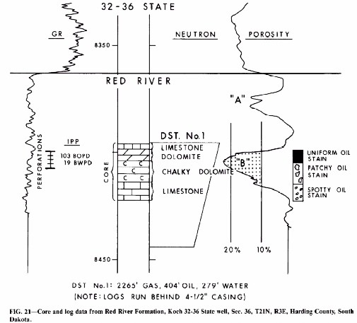
Figure 20. Map and stratigraphic cross section in west part of Buffalo field, Harding County, South Dakota.
To quantitatively interpret the free oil (type I) shows from the Clarkson well, mercury capillary pressure tests were run and studied on samples from the Koch 32-36 well. Results of these tests on three samples from the 32-36 well are illustrated on Figure 22. A capillary curve from a reservoir sample from the 14-31 Travers well is shown for comparison and is presumed to be similar to the reservoir in the 14-24 well. Inspection of these capillary curves shows that the 10% displacement pressure for the three illustrated samples from the Koch well range from 130 to 220 psi. This suggests that, for these samples to be oil stained, the minimum oil column required to force oil into these samples would be from 66 to 132 ft (20 to 40 m), using the same assumptions as used in Buffalo field example. Quantitative interpretation of the oil-stained chalky dolomite samples in the Koch 32-36, and by analog the Clarkson well, suggests that the oil-stained samples are nonreservoir or marginal reservoir rocks, and that an oil column greater than 132 ft (40 m) must be present downdip to create the observed oil staining. More accurate estimates could be made if the actual oil saturation which may be greater than 10% could be calculated from logs or other data. Quantitative studies of this type would compliment the qualitative interpretation of this test case, in that it would help define the downdip limits of the inferred large oil column.
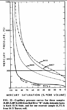
Figure 21. Core and log data from Red River Formation, Koch 32-36 State well, Sec. 36, T21N, R3E, Harding County, South Dakota.
The drill-stem test recovery of two-thirds water in the Clarkson well can also be explained quantitatively by careful examination of the inferred waste zone and the sucrosic dolomite in the good quality reservoir. Subsurface oil saturations can be read directly off the capillary pressure curve by converting the oil column to mercury pressure. To compare variations in oil saturations for different rock samples, a mercury pressure of 300 psi was used, which corresponds approximately to a 220-ft (67 m) oil column. The mercury saturation for each sample in Figure 22 is listed in Table 4. Saturation at 300 psi mercury range from 23 to 60% for the rocks from the Koch well. Based on a typical oil-water relative permeability curve (Figure 2), the relative permeability to oil for these saturations can be estimated Table 4).
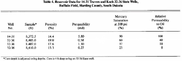
The relative permeability to oil for the three samples from the Koch 32-36 well ranges from zero to 40%. These data suggest that the fluid recovery from the oil-stained rocks in this well would be mostly water, even though the rocks have high porosity and are associated with a large oil column. The anticipated fluid recovery from quantitative show interpretation correlates closely with the actual drill-stem test recovery from the Clarkson well of 275 ft (84 m) of oil and 460 ft (140 m) of salt water. The quantitative interpretation then agrees with the qualitative interpretation previously discussed that the Clarkson well is in the waste zone of a large oil accumulation, and that if better reservoir rocks can be found downdip, they should produce mainly oil at economic rates. This concept was used in offsetting the Clarkson well downdip. The resulting well, the 14-24 Federal, has a thinner and lower porosity reservoir, yet it produces oil at an economic rate (177 bbl/day). To explain this relationship, the reservoir rocks in the 14-24 well must be similar to those studied in the core of the 14-31 Travers well. Sample examination of drill cuttings for the 14-24 well revealed sucrosic dolomite porosity in the "B" zone.
Figure 22. Capillary pressure curves for three samples (8,405,8,407,8,410) from Red River "B" chalky dolomite facies in Koch 32-36 State, and for one reservoir sample (8,372.5) from 14-31 Travers well.
Table 4. Reservoir Data for 14-31 Travers and Koch 32-36 State Wells, Buffalo Field, Harding County, South Dakota
Sample 8,372 from this well would have an oil saturation of 90% and a relative permeability to oil of 100% if associated with the same oil column as the Clarkson well (Figure 19, Table 4). This example classically illustrates the significance of reservoir pore size and permeability to the type and amount of fluid a given rock can produce. Fortunately, in this example, this drastic difference in reservoir potential can be correlated with easily recognizable rock types. The better reservoir is the sucrosic vugular large-pored dolomite, and the marginal reservoir or waste zone rock type is a chalky, earthy dolomite. The correlation between carbonate rock types and fluid recovery in this example supports ideas proposed by Archie (1952) in his paper on the classification of carbonate reservoir rocks. However, the ability to identify these two facies by sample description does not extend to log response. Note that the sucrosic dolomite sample 8,372 from the 14-31 Travers well has a core porosity of 14.4% which is similar to the maximum log porosity in the reservoir zone of the 14-24 which was not cored (Table 4). Chalky-textured dolomites from the Koch 32-36 well range from 13.3 to 19% porosity. This is illustrated on Figure 20, where the Clarkson well appears from logs to have a better reservoir than the 14-24 Federal; however, the reverse is true.
This case history example illustrates that proper interpretation of hydrocarbon shows is a valuable guide to exploration. It also demonstrates that the conventional wisdom of moving updip from a drill-stem test that recovers oil and water is not always correct.
A model for the classification and interpretation of subsurface hydrocarbon shows has been presented, which stresses the exploration and development significance of shows.
Type I (continuous phase) shows can be interpreted quantitatively. Oil or gas columns downdip from a given show can be calculated if the subsurface saturation can be determined from logs or can be estimated by comparing the minimum oil column required to explain oil shows in oil-saturated rocks and adjacent water-saturated rocks. This concept can be extremely useful in field development or in exploration, when wells can be categorized as being in the waste zone or transition zone of a complex stratigraphic trap.
Results of these research field tests suggest that estimating hydrocarbon columns from core date is a reasonably accurate and potential useful exploration tool. This approach should be particularly useful when used to compare the expected oil or gas column based on trap size predictions and the field size based on show interpretation. If an oil column is calculated significantly larger or smaller than that expected from seismic or subsurface mapping, consideration should be given to careful data review for further field development or follow-up exploration.
The settings tested in the case histories were located in areas of normal fluid pressure, hydrostatic conditions, and relatively distinct isolated stratigraphic traps with downdip water in the reservoir zone. Similar studies have been made by Berg (1975) in regard to lateral seals for stratigraphic traps. The concept of calculation of seal capacity of a given rock as used by Berg is analogous to the concept of show interpretation as presented here. Berg's quantitative results of the calculation of seal capacity agree well with the oil columns known to exist in the fields studied. Berg has also studied fields with significant downdip gravity-flow type, hydrodynamic conditions. Seal capacity interpretations in hydrodynamic settings also appear to be quantitatively accurate when compared to the oil column known to exist according to Berg (1975). This suggests that the concept of quantitative show interpretation can be extended to hydrodynamic settings with appropriate modifications for the effect of hydrodynamics on buoyancy, as defined by Berg.
This concept of interpreting hydrocarbon shows should theoretically be valid in any setting where buoyancy and capillary pressure in water-wet rocks are the primary physical forces responsible for the migration, distribution, and entrapment of bulk-phase hydrocarbons. The techniques will not be applicable in any setting where forces other than buoyancy and capillary pressure are operating. As an example, shows cannot be related to an oil or gas column where the oil or gas has been forced into the rock by processes of hydrocarbon generation and expulsion. The concept that there is a volume change during the generation of hydrocarbons allows the weight of the overburden to squeeze oil or gas out of source rocks and into any available pore space has been presented by Meissner (1978) and Momper (1978). Oil or gas shows created in this manner cannot be related to a given oil column as the oil was forced into the pore space by forces other than buoyancy.
Bulk-phase gas can also be distributed in porous rocks by forces other than buoyancy and capillary pressure, and therefore can be unrelatable to a given size gas column. Gas can be expelled from source rocks and forced into the available pore space during the gas generations and expulsion process, similar to the mechanism discussed for oil. Another gas occurrence not related to buoyant forces would be where gas in solution reaches the bubble-point saturation and begins to come out of solution. The gas bubbles would form in any available pore space and be unrelatable to a buoyant gas column. Biogenic gas released from solution may explain some of the shallow gas occurrences in tight Upper Cretaceous sandstone in Montana and North Dakota, as described by Rice and Shurr (1978). Detailed petrologic studies of the gas-bearing rocks in some of these areas indicated poor reservoir quality and very small pore size. Unusually large gas columns would be required to explain the gas occurrences in these productive rocks with very small pores and high capillary pressure if the gas is distribution controlled by the principle of buoyancy.
A third situation where gas shows may not be relatable to buoyant gas columns is in deep-basin gas fields, as those described in western Canada by Masters (1979). Follow-up work by Gies (1980) suggests that, if no downdip connected water phase is present, gas has no buoyant force, and buoyancy and capillary pressure do not control the distribution of gas. If this thesis is correct, gas shows could not be related to a given size gas column downdip because buoyancy would not be the force controlling the distribution of the gas and water.
Quantitative interpretation of hydrocarbon shows should then take into consideration the location of the show relative to mature source rocks and the possibility of quantifying an expulsion type show. The regional setting and type of gas should be considered in quantitatively interpreting any gas show to avoid interpreting bacterial gas that has come out of solution in tight gas sands and deep-basin gas occurrences that cannot be quantified by the show interpretation method.
-
Archie, G. E., 1952, Classification of carbonate reservoir rocks and petrophysical considerations: AAPG Bull., v. 36, p. 278-298.
-
Arps, J. J., 1964, Engineering concepts useful in oil finding: AAPG Bull., v. 48, p. 157-165.
-
Aufricht, W. R., and E. H. Koepf, 1957, The interpretation of capillary pressure data from carbonate reservoirs: Jour. Petroleum Technology, Oct.
-
Berg, R. R., 1975, Capillary pressure in stratigraphic traps: AAPG Bull., v. 59, p. 939-956.
-
Buckley, S. E., C. R. Hocott, and M. S. Taggart, Jr., 1958, Distribution of dissolved hydrocarbons in subsurface waters, in Habitat of oil: AAPG, p. 850-883.
-
Evans, C. R., M. A. Robers, and N. J. L. Bailey, 1971, Evolution of petroleum in western Canada: Chemical Soc., v. 8, p. 147-170.
-
Gautier, D. L., 1980, Physical characteristics of shallow methane reservoirs of northern Great Plains (abs.): AAPG Bull., v. 64, p. 711.
-
Gies, R. M., 1980, Lateral trapping mechanisms for deep basin gas trap, western Canada: AAPG Seals for Hydrocarbons Research Conf.
-
Hobson, G. D., 1962, Factors affecting oil and gas accumulations: Jour. Inst. Petroleum, v. 48, no. 461, p. 165-168.
-
Leverett, M. D., 1941, Capillary behavior in porous solids: Am. Inst. Mining and Metal. Eng. Petroleum Trans., v. 142, p. 152-169.
-
Masters, J. A., 1979, Deep basin gas trap, western Canada: AAPG Bull., v. 63, p. 152-181.
-
Meissner, F. F., 1978, Petroleum geology of the Bakken Formation, Williston basin, North Dakota and Montana: Montana Geol. Soc. Symp., p. 207-227.
-
Momper, J. A., 1978, The petroleum expulsion mechanism--a consequence of the generation process: AAPG Short Course Physical and Chemical Constraints on Petroleum Migration.
-
Prescott, M. W., 1970, Hilight field, Campbell County, Wyoming: Wyoming Geol. Assoc. Wyoming Sandstones Symp. Guidebook, p. 89-106.
-
Rice, D. D., and G. W. Shurr, 1978, Potential major natural gas resources in shallow, low permeability reservoirs of the northern Great Plains: Montana Geol. Soc. Symp., p. 265-281.
-
Salathiel, R. A., 1972, Oil recovery by surface film drainage in mixed-wettability rocks: Am. Inst. Mining, Metal., and Petroleum Eng. Petroleum Trans. SPE Paper 4104.
-
Schowalter, T. T., 1979, Mechanics of secondary hydrocarbon migration and entrapment: AAPG Bull., v. 63, p. 723-760.
-
Smith, D. A., 1966, Theoretical considerations of sealing and non-sealing faults: AAPG Bull., v. 50, p. 363-374.
-
Swanson, R. G., 1981, Sample examination manual: AAPG Methods in Exploration Series.